Creating GeoJSON out of Shapefile in R

GeoJSON has been increasingly becoming a standard format to store geospatial (geographical) information, especially for Web applications. Tools like ‘leaflet’ is making it super easy to visualize data in GeoJSON format with Java Script. And, tools like Exploratory is making it easier to visualize the data even without programming.

If you want to know more about GeoJSON, here is a great article, “More than you ever wanted to know about GeoJSON”, from Tom MacWright, which explains GeoJSON in a comprehensive and easy to digest way.

The problem is though, most of the geospatial data publicly available today are still in something called ‘Shapefile’ format, which is defined by Esri — a comapany behind one of the most popular GIS (Geographical Information System) product — and used to exchange the geospatial data among GIS softwares. It contains pretty much the same thing you find in GeoJSON, such as Polygons, Lines, Points, and their attribute information.

The good news is, converting those shapefile format files to GeoJSON format files has become much easier in R, thanks to ‘rgdal’ package from Roger Bivand and others, and the recent advancement in GeoJSON data handling with many amazing packages from ROpenSci folks.

In this post, I’m going to walk you through how you can produce your GeoJSON files out of shapefile format files and manipulate the data to fit your needs, so that you can use tools like leaflet or Exploratory, which uses leaflet internally, to quickly visualize the spatial data.

Here is the basic flow.

1. Obtain Shapefile — Geospatial (Map) Data
2. Import Shapefile to R
3. Manipulate Attributes Data in Spatial Data Frame
4. Convert to GeoJSON
5. Manipulate Geometry Data in GeoJSON — Simplify and Clip / Erase
6. Export as GeoJSON file

Install R packages for spatial and GeoJSON data handling

To do all the operations below, you will need to install the following R packages first.

• rgdal — for importing Shapefiles to R as Spatial data frame.
• spdplyr — for manipulating the attribute data inside the spatial data frame.
• geojsonio — for converting the spatial data frame to GeoJSON and saving to file systems.
• rmapshaper — for manipulating the geometry (polygon, line, marker) part of the GeoJSON data.

install.packages(rgdal)

install.packages(spdplyr)

install.packages(geojsonio)

install.packages(rmapshaper)

1. Obtain Shapefile Data Files

If you don’t have one, you can easily find the ones for what you are interested in easily on the web. Here are some examples.

US Census

This page lists many boundaries information in shapefile format like US State, Counties, Congressional Districts, etc.

GADM — Global Administrative Area

This website has built geospatial database for the world’s administrative areas (e.g. countries, province, etc.) and kindly shares the data for non-commercial use in several formats including Shapefile and RDS. And this means, you can simply import the RDS to R and skip to the step 3 without needing to deal with shapefiles at all! 👏

US National Weather Service GIS

You can find many interesting data like weather warning area, US rivers, etc, in shapefiles.

Geospatial Information Authority of Japan

You can find not only the administrative boundaries, but also something like railroads, roads, rivers, etc. in Japan.

Japan National Land Information Division GIS

This site from Japanese government lists their land management related geospatial information in shapefile format.

For this example, I’m going to use ‘US counties’ shapefile that I have downloaded from the above US Census page with this link.

2. Import Shapefile to R

Spatial Data Frame

R has a standard way to store the geospatial data with something called ‘Spatial Data Frame’, which consists of mainly two parts. One is a data frame that stores the attribute information like ID, Name, or other information. And the other part stores geometry information like polygons, which draw boundaries, lines, etc.

Import with rgdal

To import the shapefile data into R, you can use ‘readOGR’ function from ‘rgdal’ package, which is basically an R interface for gdal (Geospatial Data Abstraction Library).

library(rgdal)

county <- readOGR(dsn = "/User/kan/Data/cb_2015_us_county_500k"),

layer = "cb_2015_us_county_500k", verbose = FALSE)

The first argument is to set the path to the folder that contains all the shape files like ‘.shp’, etc. And the second is to set the name of the files without the file extension. Note that this function doesn’t like a relative path (e.g. ‘~/Data’) for ‘dsn’ argument, so you want to set an absolute path (‘/User/kan/Data’) here.

Once it’s imported, you will see a Spatial Data Frame created. If your original shape files included Polygons (Area) then you would end up with SpatialPolygonsDataFrame. If they were Lines then it would be SpatialLinesDataFrame.

You can see the attribute part of the data by adding ‘@data’ like below

# Show the first 10 rows

head(county@data, 10)

But, there is this very cool R package called ‘spdplyr’, from Michael Sumner, which basically makes it possible to use the main dplyr verbs (or functions) directly against the spatial data frames to manipulate the attribute part of the data. Also, it makes the spatial data frame to return the data in a nice table format (tibble) just by typing the spatial data frame name like below.

library(spdplyr)county

If you are a reader of this blog and a habitat of ‘tidyverse’, you will love this package. I’ll dive in more in the next section.

3. Manipulate Attribute Data, if necessary

This is not a mandatory step. If you are fine with the existing attribute information and want to generate GeoJSON with all the data, then you can skip to the next step. Otherwise, I’m listing a few scenarios where you might want to manipulate the data.

As mentioned above, thanks to ‘spdplyr’ package, you can easily manipulate the attribute part of the spatial data frame, just like you would do with dplyr commands with good ‘ol data frame.

Filtering to get only California geospatial information

Let’s say we are interested in only the counties in California. We can use filter command and set California (06) by using STATEFP column.

library(spdplyr)

county_ca <- county %>% 

  filter(STATEFP == "06")

In case, if you are not familiar with the dplyr or R basic, ‘<-’ is to store the result of the right hand side to the left hand side (county_ca). And, ‘%>%’ is to get the data of the left hand side (county) and pass it to the operation at right hand side.

Renaming the column names

If you just want to rename attribute names in the data, you can use ‘rename’ command like below.

county_id <- county %>% rename(county_id = GEOID)

Selecting or Dropping columns

There might be too many columns in your imported spatial data frame. You can select only the columns you need with ‘select’ command.

county_select <- county %>% select(STATEFP, COUNTYFP, GEOID, NAME)

As you have seen at the above examples, it’s super easy to manipulate the attribute part of the spatial data frame. Notice that the result of the manipulation is still in the spatial data frame with all the geometry information. Kudo to spdplyr! 👏

5. Manipulate Geoemtry Data in GeoJSON

This is also not mandatory step. If you are fine with the one you have, then skip to the next step.

There are two common scenarios why you might want to manipulate the geometry part of the data (e.g. Polygons, Lines, etc).

• Simplfy the geometry (Polygons, Lines) information to reduce the data size while keeping the integrity of the geometry intact.
• Keep or remove certain area of the geometry.

Here’s how.

5.1. Convert to GeoJSON

Before manipulating the geometry data, we want to convert the spatial data frame to GeoJSON first. Though you can manipulate it directly agasint the spatial data frame, I’m finding it much easier to do with GeoJSON today, thanks to amazing R packages like ‘geojsonio’ from Scott Chamberlain and ‘rmapshaper’ from Andy Teucher.

We can convert from Spatial Data Frame to GeoJSON with a function called geojson_json from geojsonio package, which makes it easy to make the geospatial data in and out of GeoJSON format.

county_json <- geojson_json(county)

The generated GeoJSON file would look something like below. (I have deleted some part of the polygon information to fit into the limited space below.)

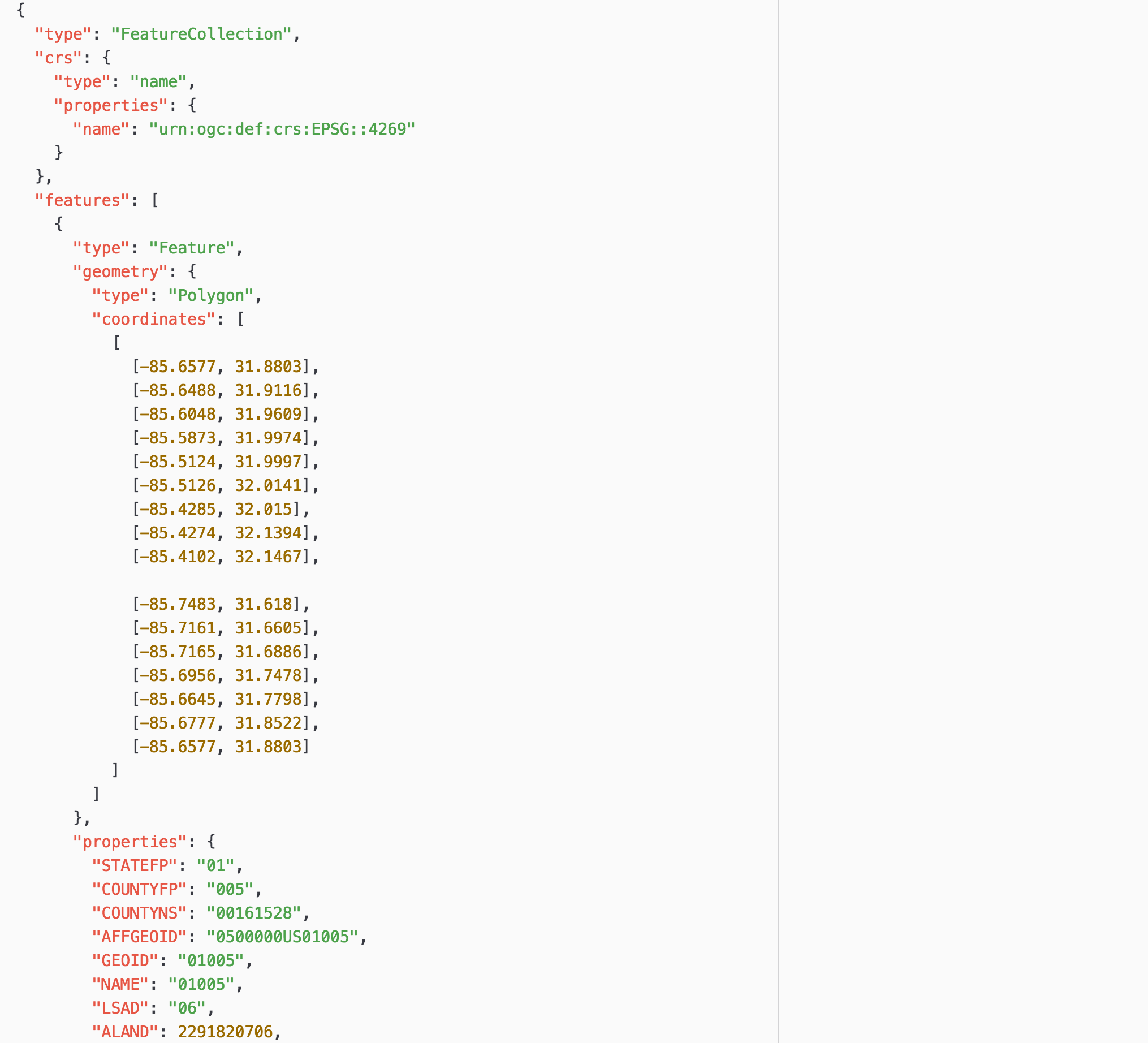
5.2. Simplify GeoJSON file

GeoJSON file size can easily get bigger because it just has a lot of information in order to draw the polygons or lines. And as you would imagine, the bigger the file size is, the slower it gets for loading, processing, and drawing the data on Map.

The good news is, you can ’simplify’ the geometry data (polygons and lines). ‘Simplify’ means that it will remove the detail information of the geometry that might not make much of the difference especially when you are visualizing the data at high level.

And even better, you can perform ‘simplify’ operation in R against GeoJSON data easily, thanks to this function called ‘ms_simpify’ from ‘rmapshaper’ package. ‘rmapshaper’ is an R interface for mapshaper library in JavaScript. It does an amazing job to reduce the data size without losing the integrity of the data. Here is how it looks before and after the ‘simplify’ operation with the default setting, which is to retain 0.05% of the original data with Visvalingam simplification algorithm.

As you can see, some areas are no longer covered by the polygons after the simplify operation. However, if you are visualizing your data by comparing among counties with color, for example, this wouldn’t make much of a difference. And the file size is now about 4MB where it used to be 27MB, that’s about 7 times smaller!

And here is the command to simplify.

library(rmapshaper)

county_json_simplified <- ms_simplify(county_json)

If you care, you can explicitly set how much you want to simplify by using ‘keep’ argument.

county_json_simplified <- ms_simplify(county_json, keep = 0.1)

5.2. Clip or Erase parts of geometry data in GeoJSON

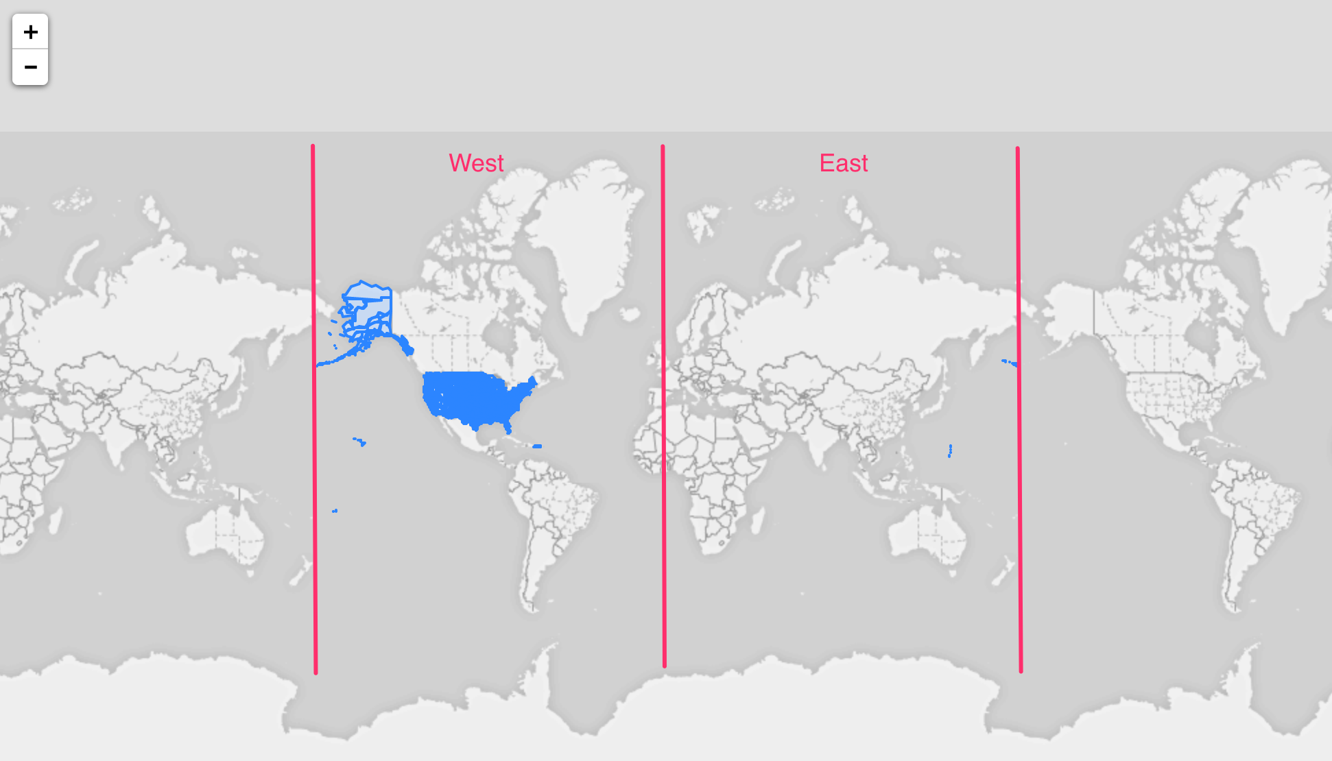
If I just use this GeoJSON file generated so far for all the counties, I would end up with a map like below.

Mapping tools like leaflet or Exploratory try to set a optimal zoom level and center position based on the available polygons or lines in the data. This means that some area of Alaska and Guam island, which are in the ‘Eastern hemisphere’ as you see in the below picture, make the tools to set the center position and zoom level in such an undesired way.

So basically, what we want in this particular case is to remove the area in Eastern hemisphere or select only the area around the main part of US within Western hemisphere. (Sorry folks in Guam, I just wanted to make things easier for this post!)

There are more than a few ways to do this in R, thanks to many amazing R packages, but so far I’m finding functions called ‘ms_clip’ and ‘ms_erase’ from the same ‘rmapshaper’ package the easiest and the most simple. ‘ms_clip’ to clip only the area we want to keep and ‘ms_erase’ to erase the area we don’t want. Here is an example with ‘ms_clip’ function.

county_json_clipped <- ms_clip(county_json_simplified, bbox = c(-170, 15, -55, 72))

The first argument is to set the GeoJSON data. The ‘bbox’ argument is to set the boundary to clip (or keep). I’m basically setting a boundary like below by setting a minimum point of longitude and latitude and a max point for the rectangle.

If you want to test out the coordinates values, you might want to use ‘lawn_bbox_polygon’ function from ‘lawn’ package like below.

library(lawn)view(lawn_bbox_polygon(c(-170, 15, -55, 72)))

This will show the boundary inside RStudio.

This ‘lawn’ package from Scott Chamberlain and others is an R interface for ‘turf.js’, which makes it easy to analyze and transform GeoJSON data. It can do a lot more amazing things, which I will explore more with future posts.

6. Export GeoJSON file

Once the GeoJSON data is ready, now we can use ‘geojson_write’ function from ‘geojsonio’ package to save (or export) it to the file system..

geojson_write(county_json_clipped, file = "~/Downloads/county.geojson")

Now, you have your own GeoJSON file and it’s time to visualize! If you are interested in visualizing your data on GeoJSON quickly, I’ve written how to do such in Exploratory in this post.

Lastly, I want to give a big shout out to ROpenSci folks who have been pushing the boundary (no pan intended!) to make Spatial data handling and analysis much more accessible to many more people including me! If you don’t know ROpenSci yet, I’d recommend this post that talks about their works in spatial area.

And also I want to thank Shinya Uryu for introducing many of the great Geospatial related R packages.

---

Entire R Script

library(rgdal)

library(geojsonio)

library(spdplyr)

library(rmapshaper)

# Import Shapefile into R.

county <- readOGR(dsn = "/Users/kan/Data/cb_2015_us_county_500k", 

                  layer = "cb_2015_us_county_500k", verbose = FALSE)

# Rename a column name GEOID to county_id.

county <- county %>% rename(county_id = GEOID)

# Convert SP Data Frame to GeoJSON.

county_json <- geojson_json(county)

# Simplify the geometry information of GeoJSON.

county_sim <- ms_simplify(county_json)

# Keep only the polygons inside the bbox (boundary box).

county_clipped <- ms_clip(county_sim, bbox = c(-170, 15, -55, 72))

# Save it to a local file system.

geojson_write(county_clipped, file = "~/Downloads/county.geojson")




For More.....